본 포스트에서는 Simple linear regression과 Non-linear regression을 tensorflow를 이용하여 구현해 볼 것입니다.
먼저 tensorflow와 numpy 라이브러리를 가져오도록 합니다.
라이브러리 가져오기
import tensorflow as tf
import numpy as np
# 버전 확인 (1.xx 버전일 경우 속도는 빠르지만 더 복잡하고 어려움)
print(tf.__version__)
Simple Linear Regression
y = ax + b 형태의 모델을 구현해 볼 것입니다.
데이터 생성
X = [1,2,3,4,5] # 입력 데이터
Y = [1,2,3,4,5] # 결과 데이터
먼저 모델에 들어가게 될 데이터 X와 Y를 생성해줍니다.
가설 정의
W = tf.Variable(tf.random.normal(shape=[1], name='weight'))
b = tf.Variable(tf.random.normal(shape=[1], name='bias'))

def hypothesis(x):    # 가설 함수 정의
    return W * x + b
가중치(weight)와 편향(bias)을 랜덤으로 설정해줍니다.
여기서 tf.Variable은 특정 값을 변수로 만들어주는 함수입니다. 이를 통해 해당 변수가 학습이 수행될 때마다 변경되어 질 수 있게 합니다.
tf.random_normal()은 평균 0, 표준편차 1인 정규분포에서 랜덤하게 초기값을 생성해줍니다. shape 옵션에 들어가는 것은 생성되는 배열의 크기를 의미합니다. (여기서는 1차원 배열이 되겠죠?)
손실 함수(cost function) 정의
def cost_fn(y_pred, y_true):
    return tf.reduce_mean(tf.square(y_pred - y_true))
손실 함수를 정의합니다. 여기서는 평균 제곱 오차(Mean Squared Error)를 사용했습니다.
최적화 알고리즘 (optimizer) 선택
optimizer = tf.optimizers.SGD(learning_rate=0.01)
cost function을 최소화하기 위해 optimizer를 정합니다.
여기서는 Stochastic Gradient Descent (SGD) 알고리즘을 사용했습니다.
모델 학습
for step in range(2000):
# tf.GradientTape() => 자동으로 미분계산
with tf.GradientTape() as g:
pred = hypothesis(X) # y = W*x + b
cost = cost_fn(pred, Y) # Loss = 1/N * sum ( square(y_pred-y_true) )
# gradient 계산
gradients = g.gradient(cost, [W,b]) # dy_dx : [cost_W, cost_b]
# gradient에 따라서 W,b 업데이트
optimizer.apply_gradients(zip(gradients, [W,b]))
# 200번째 step마다 cost, W, b 값 출력
if step % 200 == 0:
pred = hypothesis(X)
cost = cost_fn(pred, Y)
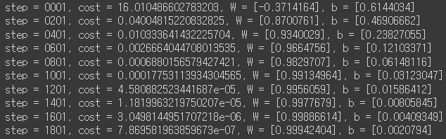
print(f'step = {step+1:0>4}, cost = {cost}, W = {W.numpy()}, b = {b.numpy()}')
tf.GradientTape()를 이용해서 자동 미분을 수행하고, SGD optimizer를 통해 W, b를 업데이트하는 과정을 2000번 반복합니다.
시각화
import matplotlib.pyplot as plt

plt.plot(X, Y, 'ro', label = 'Original Data')
plt.plot(X, np.array(W*X + b), label='Fitted Line')
plt.legend()
plt.grid()
plt.title('Linear Regression')
plt.xlabel('x')
plt.ylabel('y')
plt.show()
시각화는 matplotlib.pyplot 라이브러리를 사용하였습니다.
여기서 grid()는 그래프에 보이는 격자를 나타나게 해주는 코드이고, legend()는 범례를 나타나게 해줍니다.

예측
x_test = [10, 20, 30, 40 ,50]
x_test_predict = np.array(x_test * W + b)
print("If [10, 20, 30, 40, 50] appear, then correct!\n", x_test_predict)
테스트 데이터를 이용해 모델이 학습 데이터의 경향성(y=x)을 잘 학습했는지 측정해보겠습니다.

예측 값이 실제 값에 거의 근접하는 것으로 보아 잘 학습이 된 것으로 보입니다.
Non-Linear Regression
Simple linear regression을 구현해보았으니 이제 non-linear 형태도 구현해봐야겠죠?
저는 y = ax^2 + bx + c 형태의 비선형 모델을 구현해 볼 것입니다.
데이터 생성
X = tf.random.normal([50])	# 입력 데이터
Y = X**2 + X*tf.random.normal([50])	# 결과 데이터

X = X.numpy()
Y = Y.numpy()
모델이 학습하게 될 데이터 X와 Y를 생성해줍니다.
tf.random.normal()을 사용하여 평균 0, 표준편차 1인 정규분포에서 랜덤하게 숫자를 생성합니다. 여기서는 1차원 배열인 50개의 숫자가 X, Y에 각각 만들어질 것입니다.
X, Y는 입력, 결과 데이터이므로 tf.Tensor가 아닌 numpy 배열로 바꿔줍니다.
초기 가중치, 편향 설정
a = tf.Variable(tf.random.normal([1]))
b = tf.Variable(tf.random.normal([1]))
c = tf.Variable(tf.random.normal([1]))

# original line 기억해두기
x_ = np.arange(-5., 5., 0.001)
y_ = a*(x_)**2 + b*(x_) + c
초기 가중치(weight)와 편향(bias)을 랜덤으로 설정해줍니다. 저는 y = ax^2 + bx + c 형태를 만들 것이기 때문에 tf.Variable() 함수를 이용해 a, b, c 변수를 만들어주었습니다.
x_, y_ 변수는 랜덤으로 초기 설정된 a, b, c를 이용해 만들어진 original line을 기억해두기 위해 만들었습니다. 학습 후에 시각화 과정에서 비교 목적으로 사용될 것입니다.
가설 정의
def hypothesis(x):
  return a*(x)**2 + b*x + c
가설 함수는 y = ax^2 + bx + c 식으로 정의합니다.
손실 함수(cost function) 정의
def cost_fn(y_pred, y_true):
    return tf.reduce_mean(tf.square(y_pred - y_true))
손실 함수를 정의합니다. 위와 같이 평균 제곱 오차(Mean Squared Error)를 사용했습니다.
최적화 알고리즘 (optimizer) 선택
optimizer = tf.optimizers.Adam(learning_rate = 0.01)
cost function을 최소화하기 위해 optimizer를 정합니다.
이번에는 Adaptive Moment Estimation (Adam) 알고리즘을 사용했습니다.
모델 학습
for step in range(1,1001):
with tf.GradientTape() as g:
pred = hypothesis(X) # y = a*(x)**2 + b*x + c
cost = cost_fn(pred, Y) # Loss = 1/N * sum ( square(y_pred-y_true) )
gradients = g.gradient(cost, [a,b,c])
optimizer.apply_gradients(zip(gradients, [a,b,c]))
if step % 100 == 0:
pred = hypothesis(X)
cost = cost_fn(pred, Y)
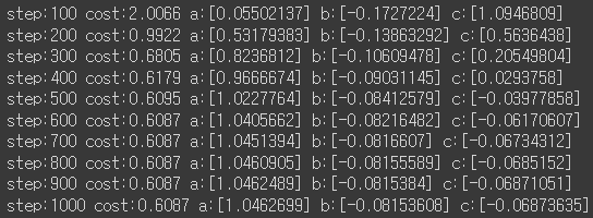
print(f" step:{step} cost:{cost:.4f} a:{a.numpy()} b:{b.numpy()} c:{c.numpy()} ")
tf.GradientTape()를 이용해서 기울기를 계산하고, Adam optimizer를 통해 계산된 기울기를 업데이트하는 과정을 1000번 반복합니다.
시각화
line_x = np.arange(min(X), max(X), 0.001)
line_y = a*(line_x)**2 + b*(line_x) + c

plt.scatter(X,Y, label = "non-linear point")
plt.plot(x_,y_, 'g', label = "original line")
plt.plot(line_x, line_y, 'r', label = "After training")
plt.legend()
plt.xlim(-5., 5)
plt.grid()
plt.show()
앞에서 만들어두었던 x_, y_를 가져와 original line을 시각화하고, 학습 후에 fit된 line과 비교해보았습니다.

학습되기 전 original line은 완전히 point들을 제대로 설명하지 못하는 것처럼 보이는 반면, 학습 후 만들어진 line은 눈으로 보기에도 non-linear point들의 경향성을 잘 나타내고 있음을 확인할 수 있습니다.
'Study > AI' 카테고리의 다른 글
| [AI] Artificial Intelligence 인공지능 입문 강의 (POSTECH 유환조 교수님) (0) | 2024.06.07 |
|---|---|
| [AI] CNN(Convolutional Neural Network)을 사용하여 MNIST 데이터 분류하기 (1) | 2024.04.10 |
| [AI] 혼동 행렬(Confusion matrix) 직접 구현하기 (0) | 2024.03.26 |
| [AI] 로지스틱 회귀(Logistic Regression) 직접 구현하기 (0) | 2024.03.25 |


