모델의 성능은 사용되는 Feature(특성)의 품질과 선택에 크게 좌우됩니다.
Feature 선택과 중요도 평가는 데이터를 분석하고 머신러닝 모델을 개발할 때, 효율적인 학습과 신뢰할 수 있는 결과를 얻기 위한 핵심 과정입니다.
본 포스팅에서는 Feature 중요도를 계산하는 주요 방법 4가지에 대해 알아보겠습니다.
- Feature Importance
- Drop-Column Importance
- Permutation Importance
- SHAP(SHapley Additive exPlanations)
데이터 셋
데이터 셋 : Adult Census Income
Adult Census Income
Predict whether income exceeds $50K/yr based on census data
www.kaggle.com
- 주제: 소득 예측 및 분류 문제
- 기반: 미국 인구 조사 데이터를 기반으로 만든 데이터셋
- 컬럼 정보:
- age: 나이
- workclass: 고용 유형 (Private, Self-emp 등)
- fnlwgt: Final Weight (가중치 변수)
- education: 학력 수준 (Bachelors, Masters 등)
- education_num: 학력 수준을 수치로 나타낸 값
- marital_status: 결혼 여부 및 상태
- occupation: 직업
- relationship: 가족 관계
- race: 인종
- sex: 성별
- capital.gain: 자본 소득
- capital.loss: 자본 손실
- hours_per_week: 주당 근무 시간
- native_country: 출생 국가
- income: 연간 소득 (목표 변수, ≤50K 또는 >50K)
1) Feature Importance (특성 중요도)
특징
- 모델이 학습하는 과정에서 각 Feature가 예측에 얼마나 기여했는지를 평가함
- 주로 트리 기반 모델(예: RandomForest, XGBoost)에 주로 사용됨
- 각 Feature가 노드 분할에 얼마나 자주 사용되었는지, 분할로 인해 감소된 불순도(Gini Impurity, Entropy 등)를 기준으로 계산
- Feature의 중요도를 상대적인 값으로 제공
장단점
장점
- 빠른 계산: 모델 학습 과정에서 Feature Importance를 자동으로 계산
- 직관적 해석: 중요도가 높은 Feature를 바로 식별
단점
- Feature 상관성 문제: 서로 상관관계가 높은 Feature가 있을 경우, 중요도가 왜곡될 수 있음(예: 중복된 Feature가 높은 중요도를 나누어 가지는 경우)
- 특정 모델에 의존: 선형 모델이나 트리 기반 모델이 아닌 경우 직접 계산이 불가
코드 (Python)
from sklearn.ensemble import RandomForestClassifier
import matplotlib.pyplot as plt

# Random Forest 모델 학습
rf = RandomForestClassifier(random_state=42)
rf.fit(X_train, y_train)

y_test_pred = rf.predict(X_test)

# feature importance 얻기
feature_importances = rf.feature_importances_

# 시각화를 위해 데이터프레임으로 만들기
importance_df = pd.DataFrame({
    'Feature': X_train.columns,
    'Importance': feature_importances
}).sort_values(by='Importance', ascending=False)

# Feature importance 시각화
plt.figure(figsize=(10, 6))
plt.barh(importance_df['Feature'], importance_df['Importance'], color='skyblue', edgecolor='black')
plt.gca().invert_yaxis()
plt.title('Feature Importance', fontsize=16)
plt.xlabel('Importance', fontsize=12)
plt.ylabel('Feature', fontsize=12)
plt.grid(axis='x', linestyle='--', alpha=0.7)
plt.show()
2) Drop-Column Importance
특징
- 각 Feature를 하나씩 제거하고 모델 성능에 미치는 영향을 측정하여 중요도를 평가하는 방식
- 모델 학습 및 예측에서 해당 Feature가 기여하는 정도를 직접적으로 확인하기 때문에 매우 직관적이고 정확한 방법
장단점
장점
- 모델 불가지론(Model-agnostic): 어떤 모델에도 적용 가능
- 정확한 중요도 계산: 각 Feature의 정확도를 직접 측정하기 때문에 가장 신뢰도가 높은 평가 방법
단점
- 높은 계산 비용: 각 Feature마다 모델을 재학습해야 하므로, Feature의 개수가 많으면 모델 학습 시간이 오래 걸림
- 데이터 의존성: 데이터 셋이 작은 경우, Feature를 제거할 때 성능 변화가 과대 또는 과소 평가될 가능성 있음
코드 (Python)
import pandas as pd
import numpy as np
from sklearn.ensemble import RandomForestClassifier
from sklearn.metrics import accuracy_score
import matplotlib.pyplot as plt

# Random Forest 모델 학습
rf = RandomForestClassifier(random_state=42)
rf.fit(X_train, y_train)

# 전체 모델의 정확도
base_accuracy = accuracy_score(y_test, rf.predict(X_test))

# Drop-Column Importance 계산
drop_importances = []

for feature in X_train.columns:
    # 해당 Feature 제거
    X_train_dropped = X_train.drop(columns=[feature])
    X_test_dropped = X_test.drop(columns=[feature])

    # 모델 재학습
    rf_dropped = RandomForestClassifier(random_state=42)
    rf_dropped.fit(X_train_dropped, y_train)

    # 정확도 계산
    dropped_accuracy = accuracy_score(y_test, rf_dropped.predict(X_test_dropped))

    # 정확도 차이로 중요도 계산
    importance = base_accuracy - dropped_accuracy
    drop_importances.append(importance)

# 데이터프레임 생성
drop_importance_df = pd.DataFrame({
    'Feature': X_train.columns,
    'Drop Importance': drop_importances
}).sort_values(by='Drop Importance', ascending=False)

# Feature Importance 시각화
plt.figure(figsize=(10, 6))
plt.barh(drop_importance_df['Feature'], drop_importance_df['Drop Importance'], color='salmon', edgecolor='black')
plt.gca().invert_yaxis()  # 가장 중요한 Feature가 상단에 위치하도록 Y축 반전
plt.title('Drop-Column Feature Importance', fontsize=16)
plt.xlabel('Decrease in Accuracy', fontsize=12)
plt.ylabel('Feature', fontsize=12)
plt.grid(axis='x', linestyle='--', alpha=0.7)
plt.tight_layout()
plt.show()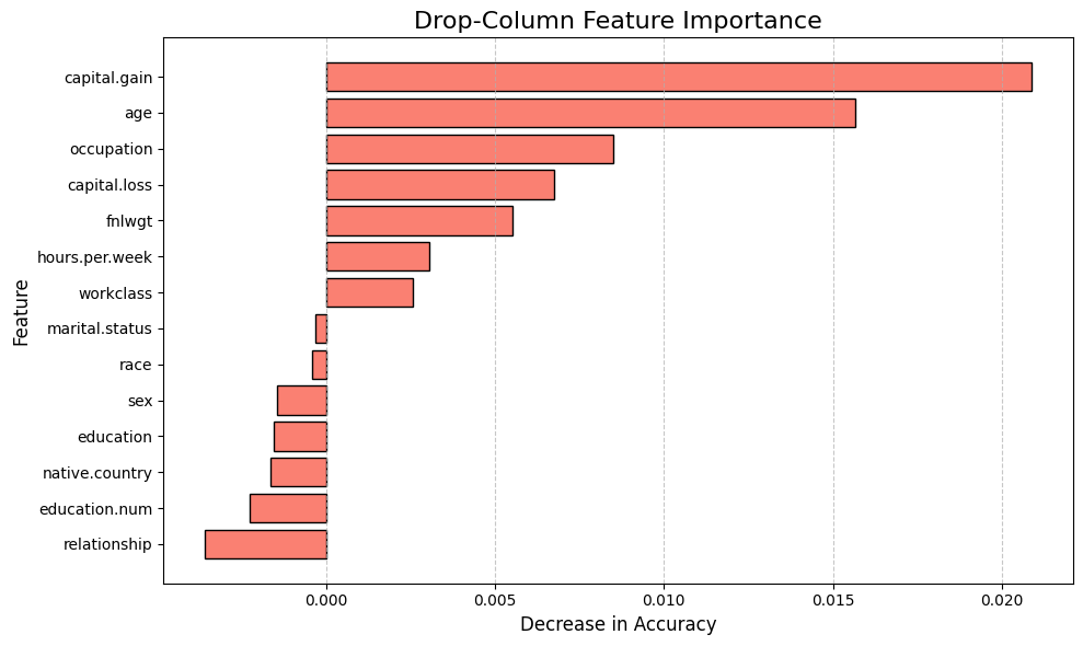
3) Permutation Importance
특징
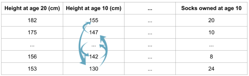
- 모델 학습 후 Feature 값을 섞어(permute) 모델 성능이 얼마나 저하되는지를 측정하여 각 Feature 중요도를 평가하는 방법
- 한 번에 한 Feature의 값을 랜덤하게 섞어 모델 예측 성능의 변화를 측정함
- 성능 변화가 클수록 해당 Feature의 중요도가 높다고 평가
장단점
장점
- 모델 불가지론(Model-agnostic): 어떤 모델에도 적용 가능
- 상관성 문제 완화: 상관성이 없는 Feature들에 대해 독립적으로 중요도를 평가하므로, 일부 상관성 문제를 해결
단점
- 높은 계산 비용: 모델을 여러 번 재평가해야 하므로, 데이터와 모델 크기에 따라 시간이 오래 걸릴 수 있음
- 랜덤성: 데이터가 랜덤으로 섞이기 때문에, 중요도가 약간 변동될 수 있음 (해결법: 여러 번 반복 후 평균 계산)
코드 (Python)
from sklearn.ensemble import RandomForestClassifier
from sklearn.inspection import permutation_importance

# Random Forest 모델 학습
rf = RandomForestClassifier(random_state=42)
rf.fit(X_train, y_train)

y_test_pred = rf.predict(X_test)

# Permutation Importance 진행
perm_importance = permutation_importance(rf, X_test, y_test, scoring="accuracy", random_state=42)

# 결과를 데이터프레임으로 만들기
importance_df = pd.DataFrame({
    "Feature": X_test.columns,
    "Importance": perm_importance["importances_mean"],
    "Std": perm_importance["importances_std"]
}).sort_values(by="Importance", ascending=False)

# Permutation Importance 시각화
plt.figure(figsize=(10, 6))
plt.barh(importance_df["Feature"], importance_df["Importance"], xerr=importance_df["Std"], color="skyblue", edgecolor="black")
plt.xlabel("Permutation Importance", fontsize=12)
plt.ylabel("Feature", fontsize=12)
plt.title("Permutation Importance", fontsize=16)
plt.gca().invert_yaxis()  # Invert Y-axis for better readability
plt.grid(axis='x', linestyle='--', alpha=0.7)
plt.show()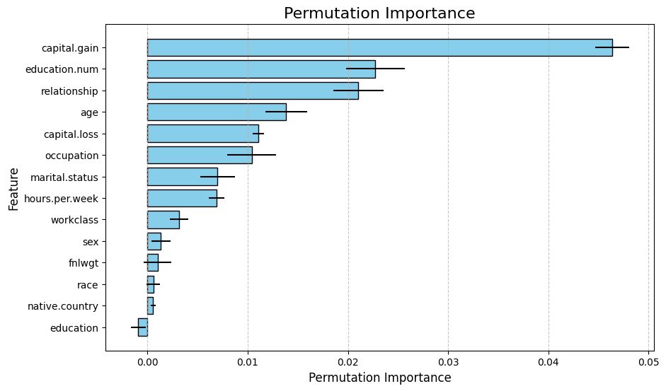
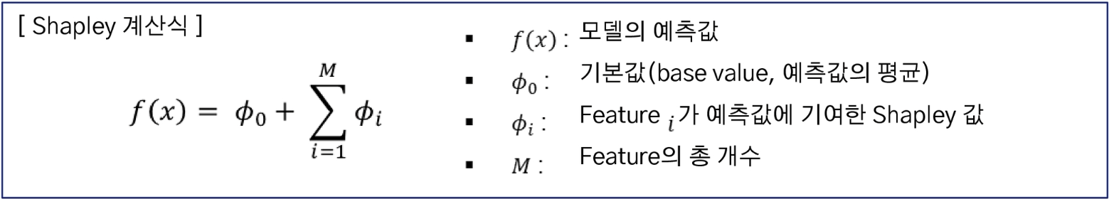
4) SHAP(SHapley Additive exPlanations)
특징
- 기계 학습 모델의 예측을 설명하기 위한 해석 가능한 인공지능(Explainable AI) 기법
- 게임 이론의 Shapley 값을 기반으로 각 Feature가 모델의 예측에 미친 영향을 정량적으로 평가함
- 특정 Feature를 포함했을 때와 포함하지 않았을 때의 모델 출력 변화를 계산하여 기여도를 평가함
- 모든 Feature 조합에 대해 반복적으로 평가하며, 결과적으로 Feature의 평균적 기여도를 계산
장단점
장점
- 모델 불가지론(Model-agnostic): 어떤 모델에도 적용 가능
- 정확한 기여도 계산: Feature의 상호작용을 고려하여 공정하게 계산
- 글로벌(Global) 해석: 모델 전체에서 어떤 Feature가 중요한지 확인
- 로컬(Local) 해석: 특정 예측값에 대해 각 Feature가 얼마나 기여했는지 분석
단점
- 높은 계산 비용: Shapley 값 계산은 조합을 반복적으로 평가해야하므로 계산 비용이 높음
- 데이터 스케일링: 모델에 따라 Feature 스케일링이 필요한 경우 SHAP 값 해석 전에 이를 고려해야 함
- 복잡한 Feature 간 상호작용 해석: SHAP은 Feature 간 상호작용을 분석할 수 있지만, 해석이 복잡할 수 있음
코드 (Python)
import shap
import matplotlib.pyplot as plt
from sklearn.ensemble import RandomForestClassifier
import pandas as pd
# 데이터 샘플링
X_sample = X_train.sample(2000, random_state=42) # 2000개 샘플만 사용
y_sample = y_train.loc[X_sample.index] # X_sample에 해당하는 타겟 값
# Random Forest 모델 학습
rf = RandomForestClassifier(random_state=42)
rf.fit(X_sample, y_sample)
# SHAP Explainer 생성
explainer = shap.Explainer(rf, X_sample)
# SHAP 값 계산
X_test_sample = X_test.iloc[:500] # 테스트 데이터에서 상위 500개 샘플만 사용
shap_values = explainer(X_test_sample, check_additivity=False)
# SHAP 값의 형식 확인 및 변환
shap_values_array = shap_values.values # NumPy 배열로 변환
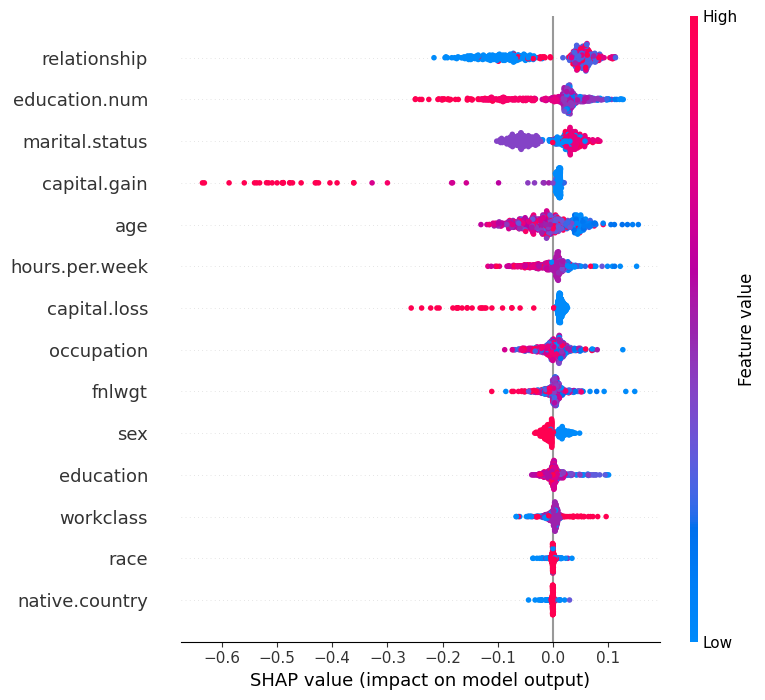
# Summary Plot
plt.figure(figsize=(8, 5))
shap.summary_plot(shap_values_array[..., 0], X_test_sample) # 첫 번째 클래스
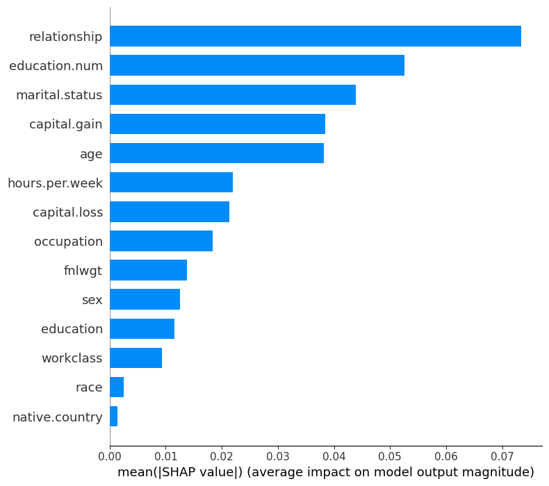
# Bar Plot
plt.figure(figsize=(8, 5))
shap.summary_plot(shap_values_array[..., 0], X_test_sample, plot_type="bar") # 첫 번째 클래스
# Force Plot (다중 클래스 분류)
index_to_explain = 0 # 첫 번째 데이터 포인트 선택
class_to_explain = 0 # 첫 번째 클래스 선택
shap.force_plot(
explainer.expected_value[class_to_explain], # 선택한 클래스의 기본값
shap_values_array[index_to_explain, :, class_to_explain], # 선택한 데이터 포인트와 클래스의 SHAP 값
X_test_sample.iloc[index_to_explain] # 선택한 데이터 포인트의 Feature 값
)
Feature 중요도 평가 방법론 비교
| 특징 | Feature Importance | Drop-Column Importance | Permutation Importance | SHAP (Shapley Additive exPlanations) |
| 평가 방식 | 트리 분할에서 불순도 감소량으로 계산 |
Feature를 제거하고 성능 변화를 측정 |
Feature 값을 섞어서 성능 변화를 관찰 |
Shapley 값을 사용하여 각 Feature가 예측값에 기여한 정도를 계산 |
| 정확도 | 대체로 정확함 | 매우 정확함 | 대체로 정확함 | 가장 높은 정확도, Feature 상호작용까지 반영 |
| 계산 비용 | 낮음 | 매우 높음 | 보통 | 보통~높음 (데이터 크기에 따라 다름) |
| 모델 의존성 | 트리 기반 모델에 한정 | 모델 불가지론 | 모델 불가지론 | 모델 불가지론 |
| 상관성 문제 | 상관성이 높은 Feature의 중요도를 과대평가할 가능성 있음 |
상관성 문제를 완화 | 상관성이 높은 Feature는 중요도 왜곡 가능 |
상관성 문제를 효과적으로 처리 가능 |
'Study > Data Science' 카테고리의 다른 글
| [Data Science] Feature(차원) 축소 - t-SNE(t-Distributed Stochastic Neighbor Embedding) (0) | 2024.12.07 |
|---|---|
| [Data Science] Feature(차원) 축소 - 주성분 분석(PCA, Principal Component Analysis) (0) | 2024.12.07 |
| [Data Science] Feature Selection - 유전 알고리즘(Genetic Algorithm, GA) (0) | 2024.12.07 |
| [Data Science] 결측 데이터 처리 방법 (3) | 2024.12.06 |


